Picking apart Perlin noise from first Principles
Although there are a lot of tutorials explaining the what and even the how of Perlin noise and the general class of algorithms; gradient noise, I have found none explaining the why behind the algorithm. Why does this algorithm work?
In this post I aim to build up perlin noise from first principles, explaining why we add each element to the algorithm as we do. We will start by trying to make a surface, perhaps for a computer game world map. We are aiming for something that looks like a mountainous region. We don’t want to hand craft this landscape as we want it to go on forever, how can we procedurally generate this world?
Given we want the surface to be random, we could start with that. However as
you can see that doesn’t lead to the most pleasing of surfaces, in fact it
wouldn’t be traversable in the game.
Our problem is that there is no smoothness from one place to another. The lowest of points could be adjacent to the highest of points. What we want is for it to take some length to go from one place to another. What we could do instead is almost zoom in on the previous example but instead of filling the point in between randomly we interpolate them. That way we could at least walk along the surface.
This leads to what is called value noise. I hope you agree it is a massive
improvement on the TV static we had in the last example.
If you look closely at this you can see quite clearly in some places where the points are from which we are interpolating. The problem here is that the gradient, the rate of change of the height can break around the edge of the interpolation. We are mapping the interpolated values 1:1 which produces a
graph as follows:

That seems fine until you put that next to another which is decreasing:

Now you get this jaring at the top. What we want is for this to be smooth. One way to do that is to make both sides of the equation have 0 gradient. That
allows you to mash them together like the following, and the smoothness is not
interrupted by breaks:


Now we know what properties we want the curve to have we need to find what the formula for this fading function is.
- We want it to go through the origin
- We want it to go through (1,1)
- We want the gradient at the origin to be flat
- We want the gradient at (1,1) to be flat
For now we are going to assume that we want a polynomial rather than using a
trig function which the mind might be drawn to by fig X.
Assuming that some polynomial will have the properties we want we can
represent it as a sum of weighted powers of x.

We want the smallest polynomial for which this is true. That is we will prefer
a quadratic over a cubic, if our requirements are met. We can see from our
requirements, specifically that we want f(0)=0 that the constant term must be
0. We can see from our requirement of the gradient at 0, f’(0)=0 that the
first power of x must also have a 0 constant.
We therefore need at least a quadratic equation. We can now search starting at
quadratic for an equation.

Unfortunately as can be seen from above it is not possible using a quadratic,
we can therefore try and use a cubic:

It works!
We now have a fade function. Applying this to our value noise we end up with
something which has less figments around the grid although looks more squarey.
It is debatable as to if this is an improvement on our last example however as
you will see, it becomes more important as we move onto our next innovation.
Introducing gradient noise
Interpolating between absolute values at the corners of the grid both before
and after our fading innovation leads to something a bit too strongly affected
by the value at the edge.
What if instead of randomly setting a value at the corners of the grid we
instead set a gradient. This way the interpolation between the corners will be
interpolating between the gradients and lead to a more interesting terrain.
For this we will represent the gradient as a vector and multiply that by the
interpolated position. I was initially a little confused by how this results
in a representation of the gradient so hopefully the following explains this a
little better.

This looks really complicated, particularly with the partial signs, but it
boils down to something quite simple.
The first line is the dot product between the two vectors, the first being the
gradients ( which we are going to pick randomly for each corner ) the second
being the position of the point we are getting a value for. The dot product is
what we are using to give us the absolute value at the point (x,y). I was
initially confused at why the first vector represents the gradient.
This can be seen from when we try to calculate the rate of change in the first
formula with a change in x. To do that we differentiate the top equation with
the assumption that y is constant. If y is constant then a1y will be constant.
When we differentiate we can throw those constants away. That leaves us with
a0. As we move along x the change in output will be a0.
The same can be seen from y.
The next question in trying to implement the noise is how do we set these
random vectors?
One way is to pick from up, down, left right randomly and that gives us a
reasonable result, far better than we managed to achieve with value noise
alone.
Choosing a vector from a list of vectors is a quick way to run the calculation
however if like here the efficiency isn’t quite so paramount, I quite like how
the result looks when the vector is chosen to be a random point on a unit
circle. Using this the angle becomes the random input and the vector of that
point becomes the output. I think this leads to less axis correlation in the
patterns.
Beyond
A lot of progress past this point has been made. One problem with this original algorithm is that for higher dimensions the number of corners which need to be interpolated from grows exponentially. This lead to the development of simplex noise which reduces the number of interpolations required by using a grid of triangles instead of squares. Ken Perlin (after whom Perlin noise is named) also extended the fade function we computed here so that the second derivative was 0 at the origin and (1,1). You can use the same logic we did here to calculate what formula that results in.
There are also a lot of tricks that can be used to produce things other than the terrain surface we originally set out to. For example, the coding train explores how to build cool loops in this video and flow fields in this one.
I want to thank http://html5gamedevelopment.com/ for providing the original javascript source code which I was able to investigate to gain a deeper understanding of how Perlin noise is calculated.


Thank you!!
ReplyDelete